We’ll look at a dataset containing popularity ratings (given by classmates) and various personal characteristics of pupils in different classes. The data are available from thecompanion website of a book on multilevel analysis (“Multilevel Analysis: Techniques and Applications, Third Edition” n.d.). The code used here borrows heavily from one of the authors’ website.
Download data
Show code
popularity <- haven::read_sav(file = "https://github.com/MultiLevelAnalysis/Datasets-third-edition-Multilevel-book/blob/master/chapter%202/popularity/SPSS/popular2.sav?raw=true")
Show code
popularity <- popularity |>
  select(-starts_with("Z"), -Cextrav, - Ctexp, -Csex) |>
  mutate(sex = haven::as_factor(sex),
         pupil = as_factor(pupil),
         class = as_factor(class))

popularity
# A tibble: 2,000 x 7
   pupil class extrav sex    texp popular popteach
   <fct> <fct>  <dbl> <fct> <dbl>   <dbl>    <dbl>
 1 1     1          5 girl     24     6.3        6
 2 2     1          7 boy      24     4.9        5
 3 3     1          4 girl     24     5.3        6
 4 4     1          3 girl     24     4.7        5
 5 5     1          5 girl     24     6          6
 6 6     1          4 boy      24     4.7        5
 7 7     1          5 boy      24     5.9        5
 8 8     1          4 boy      24     4.2        5
 9 9     1          5 boy      24     5.2        5
10 10    1          5 boy      24     3.9        3
# … with 1,990 more rows
The variables are
- pupil: ID
- class: which class are pupils in?
- extrav: extraversion score
- sex: girl or boy
- texp: teacher experience
- popular: popularity rating
- popteach: teacher popularity
- Zextrav: z-transformed extraversion score
You want to predict pupils’ popularity using their extraversion, gender and teacher experience.
It is important to consider which the predictor variables are at. extrav and sex are level-1 predictors, which means they are variables which vary with each observation (here this means by pupils), whereas texp is a level-2 predictor—this does not vary by observation, but by class. In other words, teacher experience is an attribute of class.
You should center the predictor variables.
How many pupils are there per class?
Show code
glimpse(popularity)
Rows: 2,000
Columns: 7
$ pupil    <fct> 1, 2, 3, 4, 5, 6, 7, 8, 9, 10, 11, 12, 13, 14, 15, …
$ class    <fct> 1, 1, 1, 1, 1, 1, 1, 1, 1, 1, 1, 1, 1, 1, 1, 1, 1, …
$ extrav   <dbl> 5, 7, 4, 3, 5, 4, 5, 4, 5, 5, 5, 5, 5, 5, 5, 6, 4, …
$ sex      <fct> girl, boy, girl, girl, girl, boy, boy, boy, boy, bo…
$ texp     <dbl> 24, 24, 24, 24, 24, 24, 24, 24, 24, 24, 24, 24, 24,…
$ popular  <dbl> 6.3, 4.9, 5.3, 4.7, 6.0, 4.7, 5.9, 4.2, 5.2, 3.9, 5…
$ popteach <dbl> 6, 5, 6, 5, 6, 5, 5, 5, 5, 3, 5, 5, 5, 6, 5, 5, 2, …
Show code
popularity <- popularity |>
  mutate(teacher_exp = texp - mean(texp))
Show code
popularity |>
  count(class)
# A tibble: 100 x 2
   class     n
   <fct> <int>
 1 1        20
 2 2        20
 3 3        18
 4 4        23
 5 5        21
 6 6        20
 7 7        21
 8 8        20
 9 9        20
10 10       24
# … with 90 more rows
Show code
popularity |>
  group_by(class) |>
  n_groups()
[1] 100We can plot the data, without taking into account the hierarchical structure.
Show code
popularity |>
  ggplot(aes(x = extrav,
           y = popular,
           color = class,
           group = class)) +
  geom_point(size     = 1.2,
             alpha    = .8,
             position = "jitter") +
  theme(legend.position = "none") +
  scale_color_viridis_d() +
  labs(title = "Popularity ~ Extraversion")
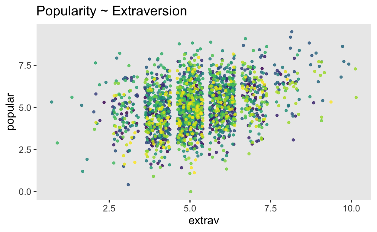
The goal here it estimate the average effect of extraversion on popularity. However, we assume that this effect will vary by class, and it might also depend on the pupils’ sex. Furthermore, classes may vary by how many years of experience a teacher has. We assume that this might be important.
Intercept-only model
Start by fitting an intercept-only model. With this we will predict
Show code
fit1 <- brm(popular ~ 1 + (1 | class),
            data = popularity,
            file = "models/pop-fit1")
In this model, we are estimating the average the average popularity over classes, as well as the deviation from this average for each class.
\[ \begin{aligned} \operatorname{popular}_{i} &\sim N \left(\alpha_{j[i]}, \sigma^2 \right) \\ \alpha_{j} &\sim N \left(\mu_{\alpha_{j}}, \sigma^2_{\alpha_{j}} \right) \text{, for class j = 1,} \dots \text{,J} \end{aligned} \]
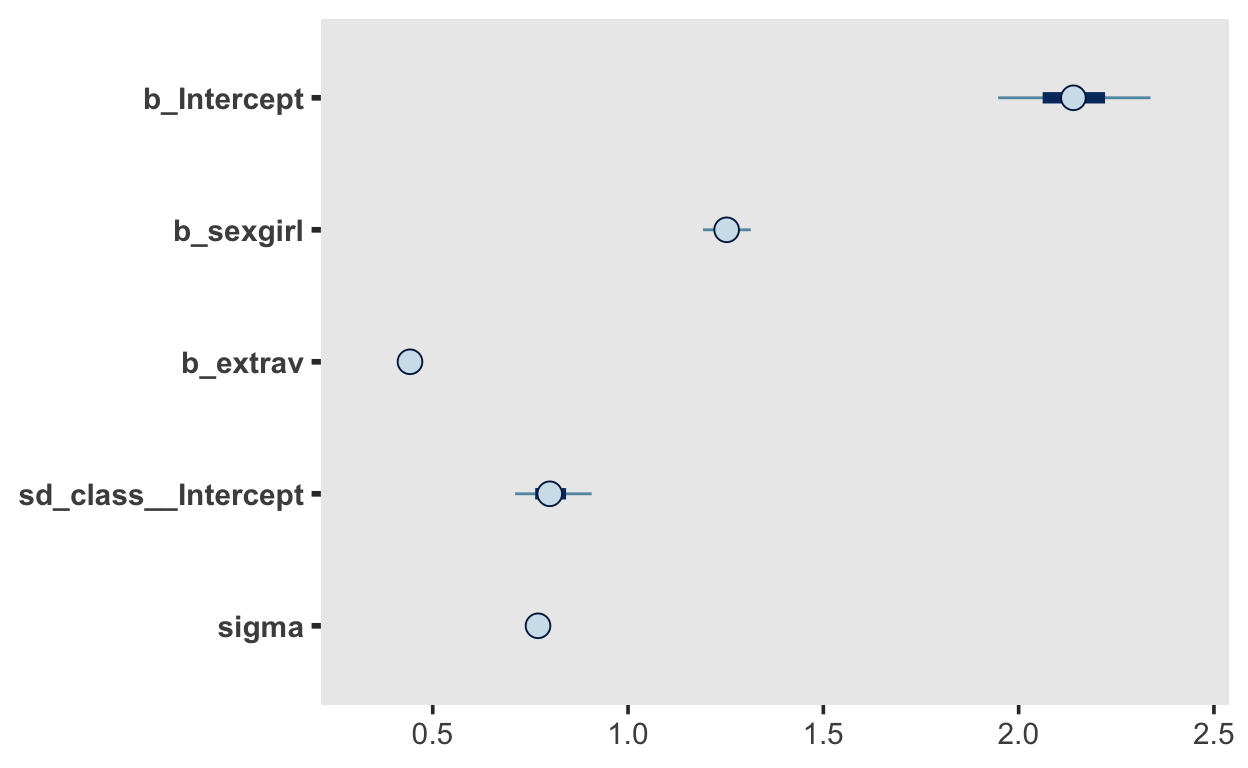
First level predictors
Now you can add some level 1 predictors, e.g. sex, extrav. You can use the update() so that you don’t have to rerun the compilation steps.
\[ \begin{aligned} \operatorname{popular}_{i} &\sim N \left(\alpha_{j[i]} + \beta_{1}(\operatorname{sex}_{\operatorname{girl}}) + \beta_{2}(\operatorname{extrav}), \sigma^2 \right) \\ \alpha_{j} &\sim N \left(\mu_{\alpha_{j}}, \sigma^2_{\alpha_{j}} \right) \text{, for class j = 1,} \dots \text{,J} \end{aligned} \]
This is equivalent to
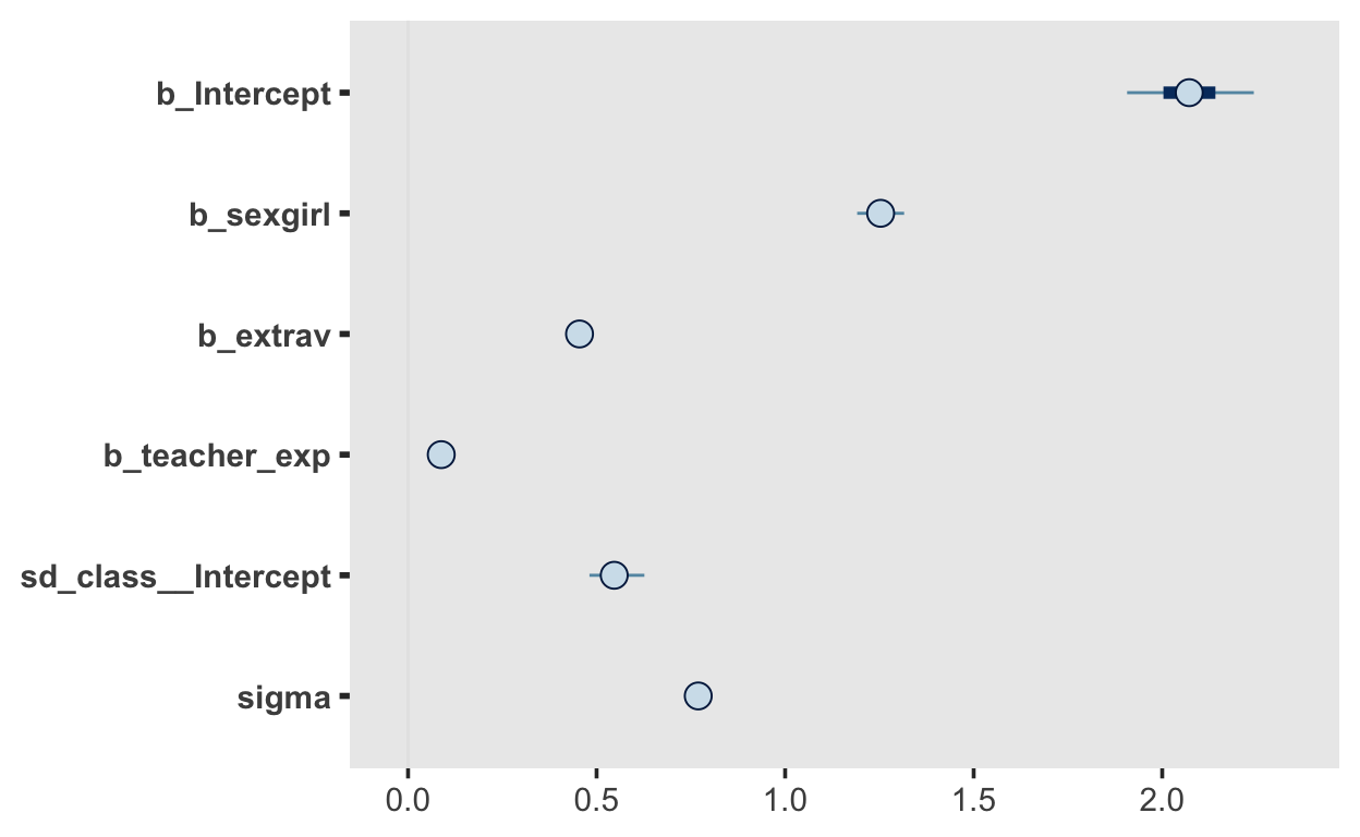
Second level predictors
Now add the the level-2 predictor teacher experience.
\[ \begin{aligned} \operatorname{popular}_{i} &\sim N \left(\alpha_{j[i]} + \beta_{1}(\operatorname{sex}_{\operatorname{girl}}) + \beta_{2}(\operatorname{extrav}), \sigma^2 \right) \\ \alpha_{j} &\sim N \left(\gamma_{0}^{\alpha} + \gamma_{1}^{\alpha}(\operatorname{teacher\_exp}), \sigma^2_{\alpha_{j}} \right) \text{, for class j = 1,} \dots \text{,J} \end{aligned} \]
Show code
fit3 <- fit2 |> update(. ~ . + teacher_exp,
                       file = "models/pop-fit3",
                       newdata = popularity)
or equivalently
Now it’s time for some plots.
Show code
fit2 |> mcmc_plot()
Show code
fit3 |> mcmc_plot()
Model comparisons
Show code
loo_compare(loo2, loo3)
     elpd_diff se_diff
fit3  0.0       0.0
fit2 -1.6       2.5
Show code
bayes_R2(fit2)
    Estimate   Est.Error      Q2.5     Q97.5
R2 0.6903738 0.006662371 0.6768908 0.7027676
Show code
bayes_R2(fit3)
    Estimate  Est.Error      Q2.5     Q97.5
R2 0.6905302 0.00680099 0.6767647 0.7035434
Show code
performance::r2_bayes(fit2)
# Bayesian R2 with Standard Error

  Conditional R2: 0.691 (89% CI [0.680, 0.701])
     Marginal R2: 0.388 (89% CI [0.372, 0.405])
Show code
performance::r2_bayes(fit3)
# Bayesian R2 with Standard Error
Conditional R2: 0.691 (89% CI [0.680, 0.701])
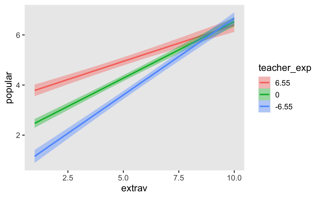
Marginal R2: 0.510 (89% CI [0.485, 0.536])Cross-level interaction
Let teacher experience interact with extraversion. This is what’s known as a cross-level interaction; extraversion is a predictor of the level 1 units (pupils), whereas teacher experience is s predictor at level 2 (classes). This can be verified by looking at the dataframe—teacher experience does not have one unique value per observation, but instead for each class.
\[ \begin{aligned} \operatorname{popular}_{i} &\sim N \left(\alpha_{j[i]} + \beta_{1}(\operatorname{sex}_{\operatorname{girl}}) + \beta_{2j[i]}(\operatorname{extrav}), \sigma^2 \right) \\ \left( \begin{array}{c} \begin{aligned} &\alpha_{j} \\ &\beta_{2j} \end{aligned} \end{array} \right) &\sim N \left( \left( \begin{array}{c} \begin{aligned} &\gamma_{0}^{\alpha} + \gamma_{1}^{\alpha}(\operatorname{teacher\_exp}) \\ &\gamma^{\beta_{2}}_{0} + \gamma^{\beta_{2}}_{1}(\operatorname{teacher\_exp}) \end{aligned} \end{array} \right) , \left( \begin{array}{cc} \sigma^2_{\alpha_{j}} & \rho_{\alpha_{j}\beta_{2j}} \\ \rho_{\beta_{2j}\alpha_{j}} & \sigma^2_{\beta_{2j}} \end{array} \right) \right) \text{, for class j = 1,} \dots \text{,J} \end{aligned} \]
Show code
conditional_effects(fit4, "extrav:teacher_exp")
You can attempt to decide which models fit better than others by using loo.