Effect of tDCS on memory
You are going to analyze data from a study in which 34 elderly subjects were given anodal (activating) tDCS over their left tempero-parietal junction (TPJ). Subjects were instructed to learn association between images and pseudo-words (data were inspired by Antonenko et al. (2019)).
Episodic memory is measured by percentage of correctly recalled word-image pairings. We also have response times for correct decisions.
Each subject was tested 5 times in the TPJ stimulation condition, and a further 5 times in a sham stimulation condition.
The variables in the dataset are:
subject: subject ID
stimulation: TPJ or sham (control)
block: block
age: age
correct: accuracy per block
rt: mean RTs for correct responses
You are mainly interested in whether recall ability is better during the TPJ stimulation condition than during sham.
Show code
d <- read_csv("https://raw.githubusercontent.com/kogpsy/neuroscicomplab/main/data/tdcs-tpj.csv")
Show code
glimpse(d)
Rows: 340
Columns: 6
$ subject     <dbl> 1, 1, 1, 1, 1, 1, 1, 1, 1, 1, 2, 2, 2, 2, 2, 2, …
$ stimulation <chr> "control", "control", "control", "control", "con…
$ block       <dbl> 1, 2, 3, 4, 5, 1, 2, 3, 4, 5, 1, 2, 3, 4, 5, 1, …
$ age         <dbl> 68, 68, 68, 68, 68, 68, 68, 68, 68, 68, 67, 67, …
$ correct     <dbl> 0.8, 0.4, 0.4, 0.4, 0.6, 0.4, 0.4, 0.6, 0.6, 0.8…
$ rt          <dbl> 1.650923, 1.537246, 1.235620, 1.671189, 1.408333…
Show code
d <- d %>%
  mutate(across(c(subject, stimulation, block), ~as_factor(.))) %>%
  drop_na()
specify a linear model
specify a null model
compare models using approximate leave-one-out cross-validation
estimate a Bayes factor for the effect of TPJ stimulation
- using the Savage-Dickey density ratio test
- using the bridge sampling method
control for subjects’ age
Linear model
Show code
summary(fit1)
Family: gaussian
Links: mu = identity; sigma = identity
Formula: correct ~ stimulation + (stimulation | subject)
Data: d (Number of observations: 315)
Samples: 4 chains, each with iter = 2000; warmup = 1000; thin = 1;
total post-warmup samples = 4000
Group-Level Effects:
~subject (Number of levels: 34)
Estimate Est.Error l-95% CI u-95% CI
sd(Intercept) 0.04 0.02 0.00 0.08
sd(stimulationTPJ) 0.03 0.02 0.00 0.08
cor(Intercept,stimulationTPJ) -0.12 0.56 -0.96 0.93
Rhat Bulk_ESS Tail_ESS
sd(Intercept) 1.00 1063 1691
sd(stimulationTPJ) 1.00 1773 1704
cor(Intercept,stimulationTPJ) 1.00 2638 2093
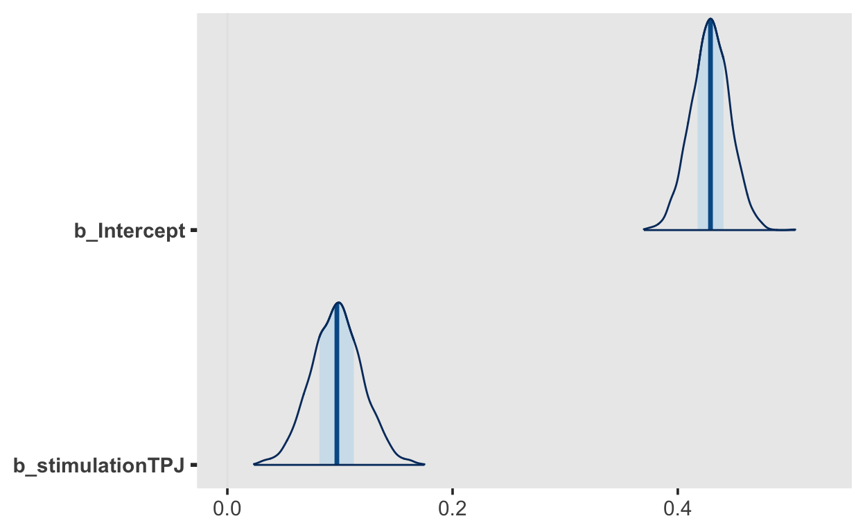
Population-Level Effects:
Estimate Est.Error l-95% CI u-95% CI Rhat Bulk_ESS
Intercept 0.43 0.02 0.39 0.46 1.00 4370
stimulationTPJ 0.10 0.02 0.05 0.14 1.00 5662
Tail_ESS
Intercept 2819
stimulationTPJ 2553
Family Specific Parameters:
Estimate Est.Error l-95% CI u-95% CI Rhat Bulk_ESS Tail_ESS
sigma 0.19 0.01 0.18 0.21 1.00 4488 2904
Samples were drawn using sampling(NUTS). For each parameter, Bulk_ESS
and Tail_ESS are effective sample size measures, and Rhat is the potential
scale reduction factor on split chains (at convergence, Rhat = 1).Show code
mcmc_plot(fit1, "b_", type = "areas")
Null model
Show code
fit2 <- brm(correct ~ 1 + (stimulation| subject),
            data = d,
            file = "models/ass4-2")
Model comparison using loo
Show code
loo_fit_1 <- loo(fit1)
loo_fit_1
Computed from 4000 by 315 log-likelihood matrix

         Estimate   SE
elpd_loo     62.3 11.3
p_loo        14.4  1.1
looic      -124.7 22.6
------
Monte Carlo SE of elpd_loo is 0.1.

All Pareto k estimates are good (k < 0.5).
See help('pareto-k-diagnostic') for details.
Show code
loo_fit_2 <- loo(fit2)
loo_fit_2
Computed from 4000 by 315 log-likelihood matrix

         Estimate   SE
elpd_loo     54.3 10.8
p_loo        17.0  1.3
looic      -108.5 21.7
------
Monte Carlo SE of elpd_loo is 0.1.

Pareto k diagnostic values:
                         Count Pct.    Min. n_eff
(-Inf, 0.5]   (good)     313   99.4%   1428
 (0.5, 0.7]   (ok)         2    0.6%   1509
   (0.7, 1]   (bad)        0    0.0%   <NA>
   (1, Inf)   (very bad)   0    0.0%   <NA>

All Pareto k estimates are ok (k < 0.7).
See help('pareto-k-diagnostic') for details.
Show code
loo_compare(loo_fit_1, loo_fit_2)
     elpd_diff se_diff
fit1  0.0       0.0
fit2 -8.1       3.7
Model comparison via Bayes factor
Show code
loglik_1 <- bridge_sampler(fit1_bf, silent = TRUE)
loglik_2 <- bridge_sampler(fit2_bf, silent = TRUE)
Show code
BF_10 <- bayes_factor(loglik_1, loglik_2)
BF_10
Estimated Bayes factor in favor of x1 over x2: 116.01251Control for age
Show code
fit3
 Family: gaussian
  Links: mu = identity; sigma = identity
Formula: correct ~ stimulation + age + (stimulation | subject)
   Data: d (Number of observations: 315)
Samples: 4 chains, each with iter = 2000; warmup = 1000; thin = 1;
         total post-warmup samples = 4000

Group-Level Effects:
~subject (Number of levels: 34)
                              Estimate Est.Error l-95% CI u-95% CI
sd(Intercept)                     0.03      0.02     0.00     0.07
sd(stimulationTPJ)                0.03      0.02     0.00     0.08
cor(Intercept,stimulationTPJ)    -0.07      0.56    -0.95     0.92
                              Rhat Bulk_ESS Tail_ESS
sd(Intercept)                 1.00     1066     1325
sd(stimulationTPJ)            1.00     1476     2197
cor(Intercept,stimulationTPJ) 1.00     2435     1959

Population-Level Effects:
               Estimate Est.Error l-95% CI u-95% CI Rhat Bulk_ESS
Intercept          0.16      0.25    -0.33     0.64 1.00     4074
stimulationTPJ     0.10      0.02     0.05     0.14 1.00     5234
age                0.00      0.00    -0.00     0.01 1.00     4075
               Tail_ESS
Intercept          2701
stimulationTPJ     2720
age                2688

Family Specific Parameters:
      Estimate Est.Error l-95% CI u-95% CI Rhat Bulk_ESS Tail_ESS
sigma     0.19      0.01     0.18     0.21 1.00     3919     2810

Samples were drawn using sampling(NUTS). For each parameter, Bulk_ESS
and Tail_ESS are effective sample size measures, and Rhat is the potential
scale reduction factor on split chains (at convergence, Rhat = 1).
Show code
loo_fit_3 <- loo(fit3)
Show code
loo_compare(loo_fit_1, loo_fit_3)
     elpd_diff se_diff
fit1  0.0       0.0
fit3 -0.4       1.0
Show code
loglik_3 <- bridge_sampler(fit3_bf, silent = TRUE)
Show code
BF_01 <- bayes_factor(loglik_3, loglik_1)
BF_01
Estimated Bayes factor in favor of x1 over x2: 0.00668