library(kableExtra)
library(viridis)
library(tidyverse)
library(brms)

# set ggplot theme
theme_set(theme_grey(base_size = 14) +
            theme(panel.grid = element_blank()))

# set rstan options
rstan::rstan_options(auto_write = TRUE)
options(mc.cores = 4)
Check out this interactive web app for response time distributions (Lindeløv 2021).
We will try to fit a distributin that is appropriate for response times to data from Wagenmakers and Brown (2007).
Subjects performed a lexical decision task in two conditions (speed stress / accuracy stress). We will look at conly correct responses.
library(rtdists)
data(speed_acc)

speed_acc <- speed_acc %>%
  as_tibble()


df_speed_acc <- speed_acc %>%
   # remove rts under 180 ms and over 3 sec
  filter(rt > 0.18, rt < 3) %>%
   # convert to char
  mutate(across(c(stim_cat, response), as.character)) %>%
  # Kcorrect responses
  filter(response != 'error', stim_cat == response) %>%
  # convert back to factor
  mutate(across(c(stim_cat, response), as_factor))
df_speed_acc
# A tibble: 27,936 x 9
id block condition stim stim_cat frequency response rt
<fct> <fct> <fct> <fct> <fct> <fct> <fct> <dbl>
1 1 1 speed 5015 nonword nw_low nonword 0.7
2 1 1 speed 6481 nonword nw_very_low nonword 0.46
3 1 1 speed 3305 word very_low word 0.455
4 1 1 speed 4468 nonword nw_high nonword 0.773
5 1 1 speed 1047 word high word 0.39
6 1 1 speed 5036 nonword nw_low nonword 0.603
7 1 1 speed 1111 word high word 0.435
8 1 1 speed 6561 nonword nw_very_low nonword 0.524
9 1 1 speed 1670 word high word 0.427
10 1 1 speed 6207 nonword nw_very_low nonword 0.456
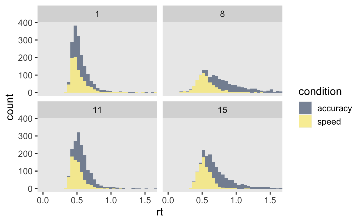
# … with 27,926 more rows, and 1 more variable: censor <lgl>Plot a few subjects to get an overview.
data_plot <- df_speed_acc %>%
  filter(id %in% c(1, 8, 11, 15))

data_plot %>%
  ggplot(aes(x = rt)) +
    geom_histogram(aes(fill = condition), alpha = 0.5, bins = 60) +
    facet_wrap(~id) +
    coord_cartesian(xlim=c(0, 1.6)) +
    scale_fill_viridis(discrete = TRUE, option = "E")
Shifted Lognormal
We’ll not try to fit a shifted-lognormal distribution
The density is given by:
\[ f(x) = \frac{1} {(x - \theta)\sigma\sqrt{2\pi}} exp\left[ -\frac{1}{2} \left(\frac{ln(x - \theta) - \mu }{\sigma} \right)^2 \right] \]
m\(\mu\), \(\sigma\) und \(\theta\) are the three parameters. \(\theta\) shifts the entire distribition along the x axis. \(\mu\) and \(\sigma\) have an effect on the shape.
\(\mu\) is often interpreted as a difficulty parameter. Both median and mean depend on \(\mu\)
The median is given by \(\theta + exp(\mu)\).
\(\sigma\) is the scale parameter (standard deviation); It affects the mean, but not the median.
The mean is \(\theta + exp\left( \mu + \frac{1}{2}\sigma^2\right)\)
We are mainly interested in the \(\mu\) parameter.
When fitting with brms, we need to be aware that \(\mu\) and \(\sigma\) are on the log scale.
\[ y_i \sim Shifted Lognormal(\mu, \sigma, \theta) \]
\[ log(\mu) = b_0 + b_1 X_1 + ...\] Both \(\sigma\) and \(\theta\) may also be predicted, or simply estimated.
\[ \sigma \sim Dist(...) \]
\[ \theta \sim Dist(...) \]
priors <- get_prior(rt ~ condition + (1|id),
          family = shifted_lognormal(),
          data = df_speed_acc)

priors %>%
  as_tibble() %>%
  select(1:4)
# A tibble: 8 x 4
  prior                     class     coef             group
  <chr>                     <chr>     <chr>            <chr>
1 ""                        b         ""               ""
2 ""                        b         "conditionspeed" ""
3 "student_t(3, -0.6, 2.5)" Intercept ""               ""
4 "uniform(0, min_Y)"       ndt       ""               ""
5 "student_t(3, 0, 2.5)"    sd        ""               ""
6 ""                        sd        ""               "id"
7 ""                        sd        "Intercept"      "id"
8 "student_t(3, 0, 2.5)"    sigma     ""               ""
priors <- prior(normal(0, 0.1), class = b)
m1 <- brm(rt ~ condition + (1|id),
          family = shifted_lognormal(),
          prior = priors,
          data = df_speed_acc,
          file = 'models/m1_shiftedlognorm')
summary(m1)
 Family: shifted_lognormal
  Links: mu = identity; sigma = identity; ndt = identity
Formula: rt ~ condition + (1 | id)
   Data: df_speed_acc (Number of observations: 27936)
Samples: 4 chains, each with iter = 2000; warmup = 1000; thin = 1;
         total post-warmup samples = 4000

Group-Level Effects:
~id (Number of levels: 17)
              Estimate Est.Error l-95% CI u-95% CI Rhat Bulk_ESS
sd(Intercept)     0.15      0.03     0.11     0.23 1.01      467
              Tail_ESS
sd(Intercept)      736

Population-Level Effects:
               Estimate Est.Error l-95% CI u-95% CI Rhat Bulk_ESS
Intercept         -0.68      0.04    -0.76    -0.61 1.01      455
conditionspeed    -0.40      0.00    -0.41    -0.39 1.00     1766
               Tail_ESS
Intercept           594
conditionspeed     1707

Family Specific Parameters:
      Estimate Est.Error l-95% CI u-95% CI Rhat Bulk_ESS Tail_ESS
sigma     0.37      0.00     0.36     0.37 1.00     1863     2071
ndt       0.17      0.00     0.17     0.18 1.00     1479     2166

Samples were drawn using sampling(NUTS). For each parameter, Bulk_ESS
and Tail_ESS are effective sample size measures, and Rhat is the potential
scale reduction factor on split chains (at convergence, Rhat = 1).
# intial values for expected ndt
inits <- function() {
list(Intercept_ndt = -1.7)
}
m2 <- brm(bf(rt ~ condition + (1|id),
ndt ~ 1 + (1|id)),
family = shifted_lognormal(),
prior = priors,
data = df_speed_acc,
inits = inits,
init_r = 0.05,
control = list(max_treedepth = 12),
file = 'models/m2_shiftedlognorm_ndt')
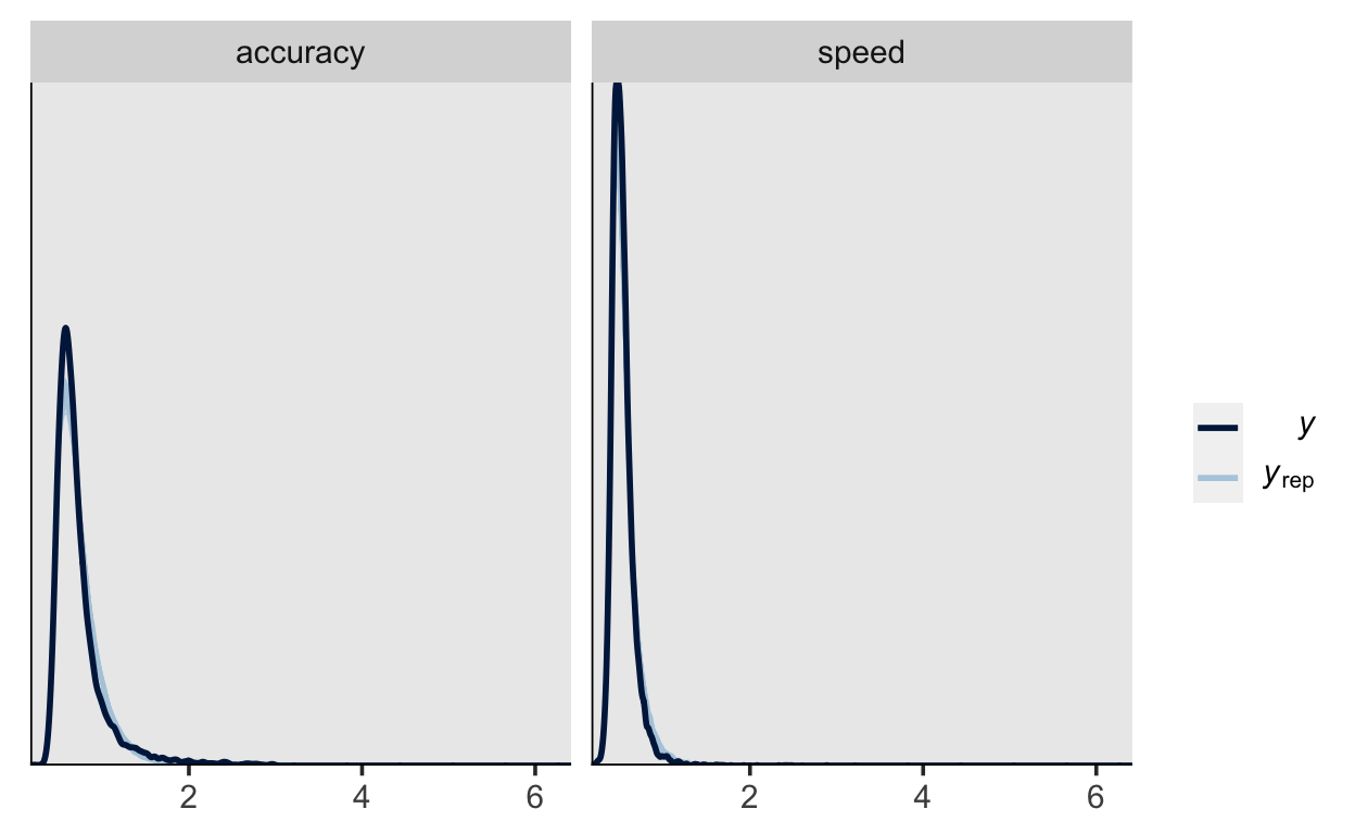
pp_check(m2,
         type = "dens_overlay_grouped",
         group = "condition",
         nsamples = 200)