Learn multilevel models: Longitudinal Models

Andrew Ellis

The examples in this document are taken from Singer and Willett (n.d.) and the translation into tidyverse and brms code by Kurz (2021).

We will first briefly look at how to reshape datasets, and then investigate two examples of longitudinal data with a hierarchical structure.

library(kableExtra)
library(tidyverse)
library(brms)

# set ggplot theme
theme_set(theme_grey(base_size = 14) +
            theme(panel.grid = element_blank()))

# set rstan options
rstan::rstan_options(auto_write = TRUE)
options(mc.cores = 4)

Exploring data

We’ll load a dataset from RAUDENBUSH and CHAN (1992).

tolerance <- read_csv("https://stats.idre.ucla.edu/wp-content/uploads/2016/02/tolerance1.txt", col_names = TRUE)

head(tolerance, n = 16)

# A tibble: 16 x 8
      id tol11 tol12 tol13 tol14 tol15  male exposure
   <dbl> <dbl> <dbl> <dbl> <dbl> <dbl> <dbl>    <dbl>
 1     9  2.23  1.79  1.9   2.12  2.66     0     1.54
 2    45  1.12  1.45  1.45  1.45  1.99     1     1.16
 3   268  1.45  1.34  1.99  1.79  1.34     1     0.9 
 4   314  1.22  1.22  1.55  1.12  1.12     0     0.81
 5   442  1.45  1.99  1.45  1.67  1.9      0     1.13
 6   514  1.34  1.67  2.23  2.12  2.44     1     0.9 
 7   569  1.79  1.9   1.9   1.99  1.99     0     1.99
 8   624  1.12  1.12  1.22  1.12  1.22     1     0.98
 9   723  1.22  1.34  1.12  1     1.12     0     0.81
10   918  1     1     1.22  1.99  1.22     0     1.21
11   949  1.99  1.55  1.12  1.45  1.55     1     0.93
12   978  1.22  1.34  2.12  3.46  3.32     1     1.59
13  1105  1.34  1.9   1.99  1.9   2.12     1     1.38
14  1542  1.22  1.22  1.99  1.79  2.12     0     1.44
15  1552  1     1.12  2.23  1.55  1.55     0     1.04
16  1653  1.11  1.11  1.34  1.55  2.12     0     1.25

The data are in the wide format (one row per id), but we need one row per observation, so we need to rehape the data into a long format.

tolerance <- tolerance |> 
  pivot_longer(-c(id, male, exposure),
               names_to = "age", 
               values_to = "tolerance") |> 
  # remove the `tol` prefix from the `age` values 
  mutate(age = str_remove(age, "tol") |> as.integer()) |> 
  arrange(id, age)

We have 16 subjects.

tolerance %>% 
  distinct(id) %>% 
  count()

# A tibble: 1 x 1
      n
  <int>
1    16

tolerance %>%
  slice(c(1:9, 76:80))

# A tibble: 14 x 5
      id  male exposure   age tolerance
   <dbl> <dbl>    <dbl> <int>     <dbl>
 1     9     0     1.54    11      2.23
 2     9     0     1.54    12      1.79
 3     9     0     1.54    13      1.9 
 4     9     0     1.54    14      2.12
 5     9     0     1.54    15      2.66
 6    45     1     1.16    11      1.12
 7    45     1     1.16    12      1.45
 8    45     1     1.16    13      1.45
 9    45     1     1.16    14      1.45
10  1653     0     1.25    11      1.11
11  1653     0     1.25    12      1.11
12  1653     0     1.25    13      1.34
13  1653     0     1.25    14      1.55
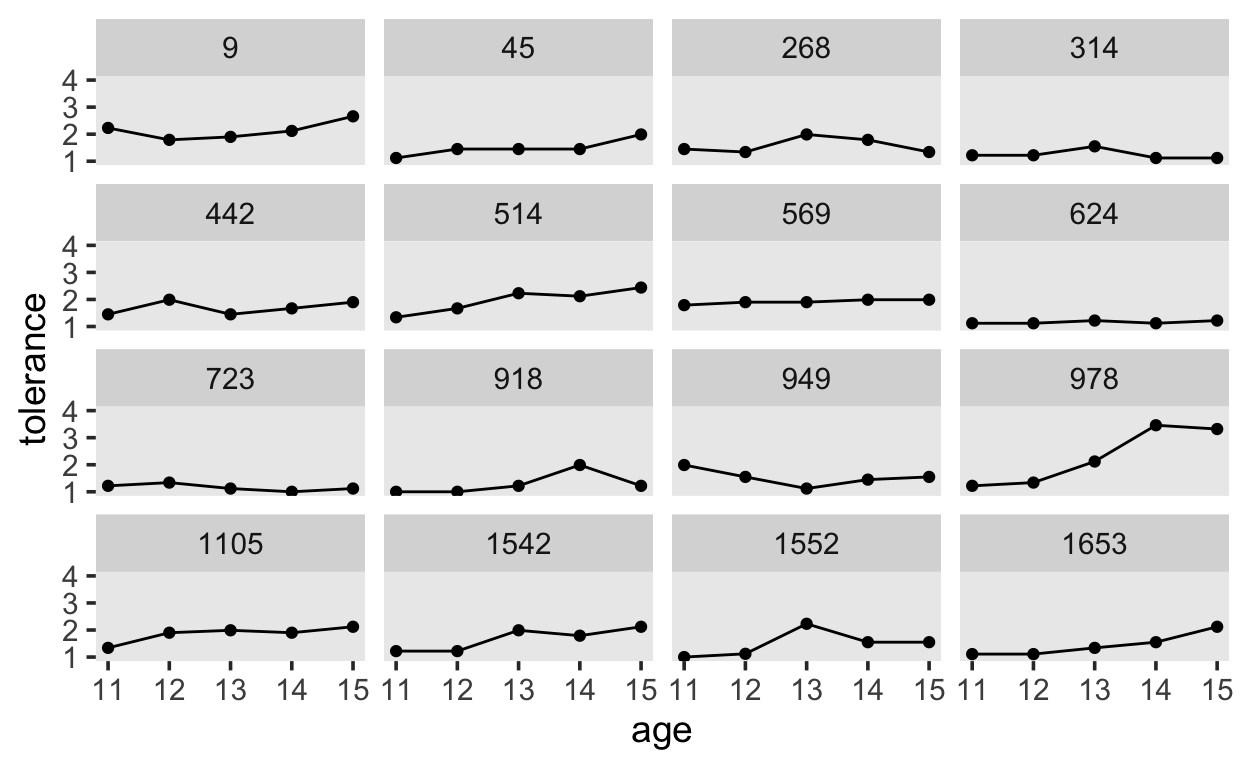
14  1653     0     1.25    15      2.12

First, we will plot the observations over time (at different ages), and connect them with lines.

tolerance %>%
  ggplot(aes(x = age, y = tolerance)) +
  geom_point() +
  geom_line() +
  coord_cartesian(ylim = c(1, 4)) +
  theme(panel.grid = element_blank()) +
  facet_wrap(~id)

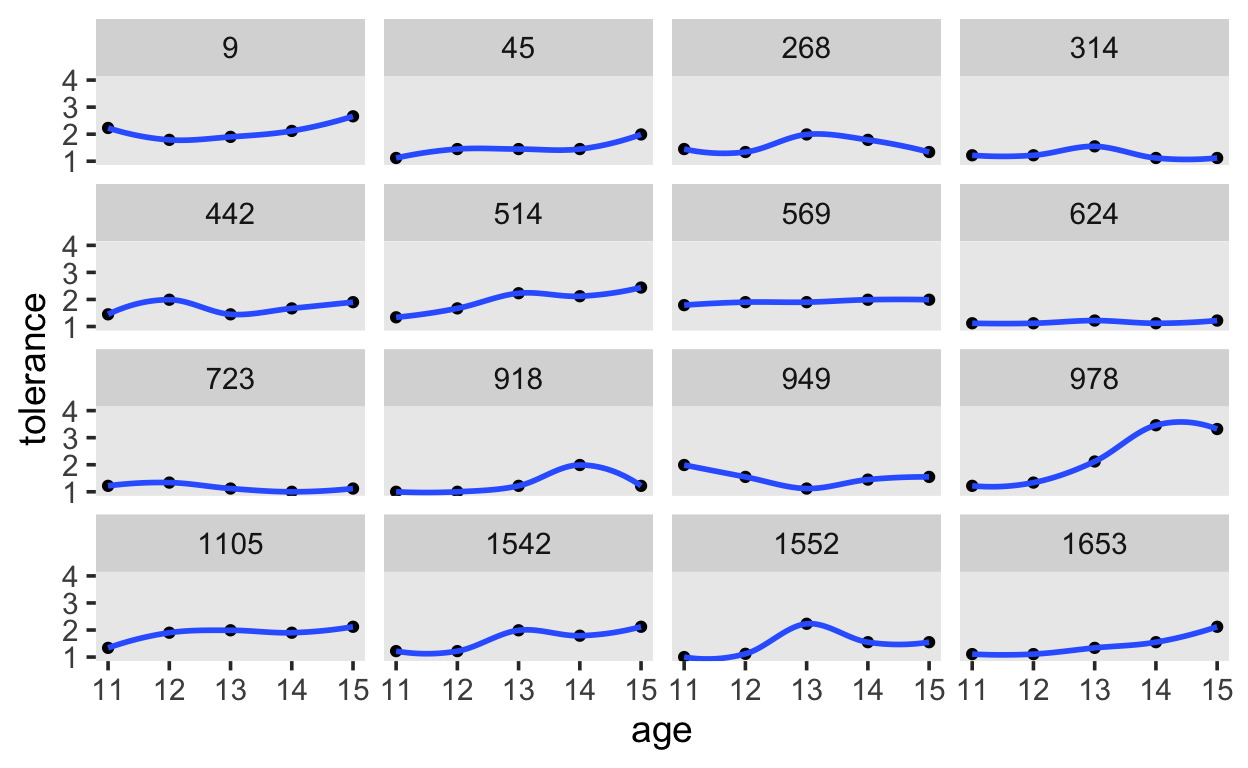
Next, we will apply locally weighted smoothing.

tolerance %>%
  ggplot(aes(x = age, y = tolerance)) +
  geom_point() +
  stat_smooth(method = "loess", se = F, span = .9) +
  coord_cartesian(ylim = c(1, 4)) +
  theme(panel.grid = element_blank()) +
  facet_wrap(~id)

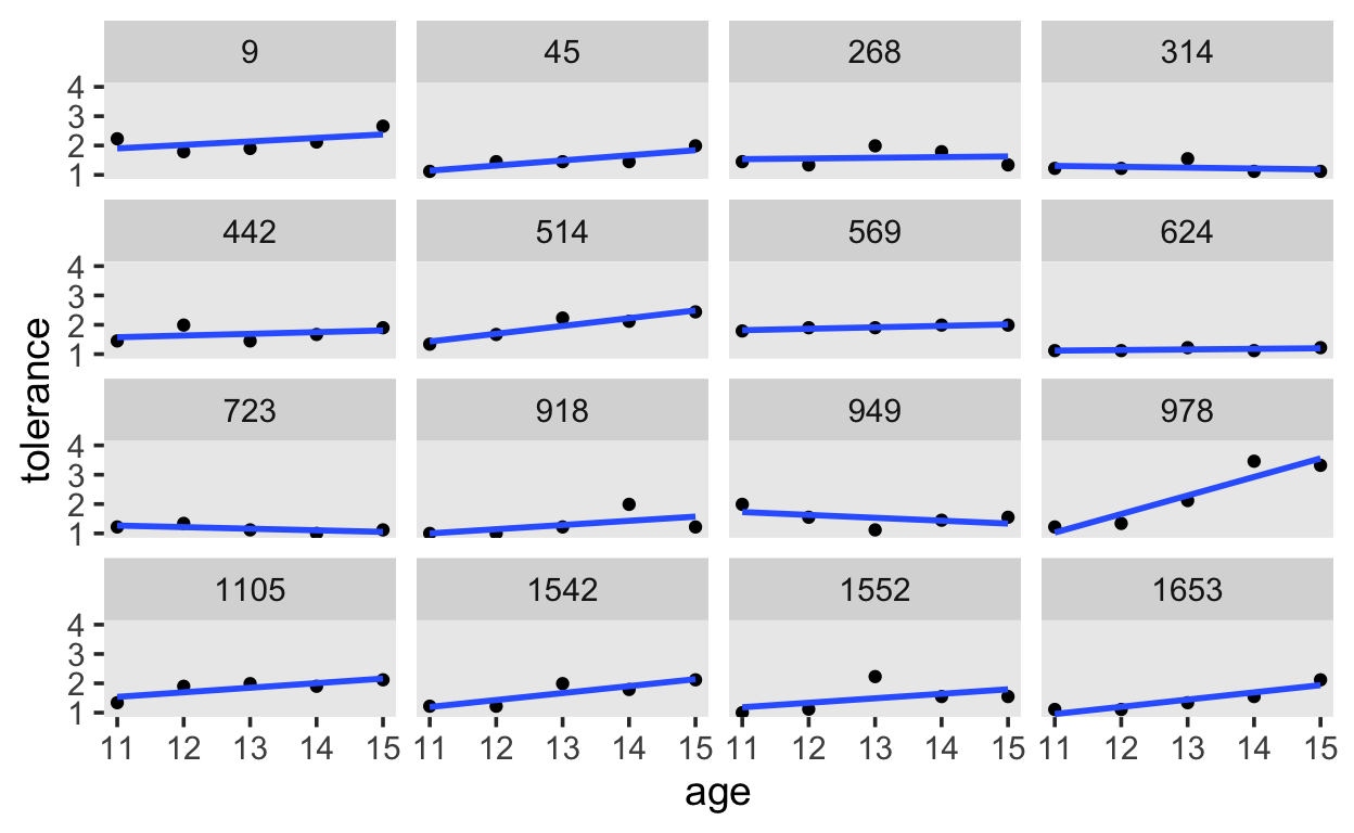
And finally, we’ll estimate the linear effect of age.

tolerance %>%
  ggplot(aes(x = age, y = tolerance)) +
  geom_point() +
  stat_smooth(method = "lm", se = F, span = .9) +
  coord_cartesian(ylim = c(1, 4)) +
  theme(panel.grid = element_blank()) +
  facet_wrap(~id)

Early Intervention

We’ll start with a data set on early intervention on child development (Singer and Willett n.d.)

As part of a larger study of the effects of early intervention on child development, these researchers tracked the cognitive performance of 103 African- American infants born into low-income families. When the children were 6 months old, approximately half (n = 58) were randomly assigned to participate in an intensive early intervention program designed to enhance their cognitive functioning; the other half (n = 45) received no intervention and constituted a control group. Each child was assessed 12 times between ages 6 and 96 months. Here, we examine the effects of program participation on changes in cognitive performance as measured by a nationally normed test administered three times, at ages 12, 18, and 24 months.

Each child has three records, one per wave of data collection. Each record contains four variables: (1) ID; (2) AGE, the child’s age (in years) at each assessment (1.0, 1.5, or 2.0); (3) COG, the child’s cognitive performance score at that age; and (4) PROGRAM, a dichotomy that describes whether the child participated in the early intervention program. Because children remained in their group for the duration of data collection, this predictor is time-invariant.

early_int <- read_csv("https://raw.githubusercontent.com/awellis/learnmultilevelmodels/main/data/early-intervention.csv") |> 
  mutate(id = as_factor(id),
         intervention = factor(ifelse(program == 0, "no", "yes"),
                               levels = c("no", "yes")))

head(early_int, 10)

# A tibble: 10 x 6
   id      age   cog program age_c intervention
   <fct> <dbl> <dbl>   <dbl> <dbl> <fct>       
 1 1       1     117       1   0   yes         
 2 1       1.5   113       1   0.5 yes         
 3 1       2     109       1   1   yes         
 4 2       1     108       1   0   yes         
 5 2       1.5   112       1   0.5 yes         
 6 2       2     102       1   1   yes         
 7 3       1     112       1   0   yes         
 8 3       1.5   113       1   0.5 yes         
 9 3       2      85       1   1   yes         
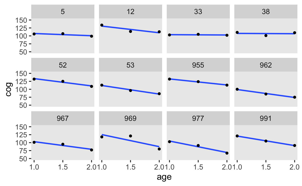
10 4       1     138       1   0   yes

In addition, we have the age-1 variable, age_c. This variable has the value 0 when the child is 1 year old.

early_int |> 
  filter(id %in% sample(levels(early_int$id), 12)) |> 
  ggplot(aes(x = age, y = cog)) +
  stat_smooth(method = "lm", se = F) +
  geom_point() +
  scale_x_continuous(breaks = c(1, 1.5, 2)) +
  ylim(50, 150) +
  theme(panel.grid = element_blank()) +
  facet_wrap(~id, ncol = 4)

Our model for each child’s development is:

\[ \text{cog}_{ij} = [ \pi_{0i} + \pi_{1i} (\text{age}_{ij} - 1) ] + [\epsilon_{ij}]. \]

\[\begin{align*} \text{cog} & \sim \operatorname{Normal} (\mu_{ij}, \sigma_\epsilon^2) \\ \mu_{ij} & = \pi_{0i} + \pi_{1i} (\text{age}_{ij} - 1). \end{align*}\]

The \(i^{th}\) child’s cog score at observation \(j\) is normally distributed, with mean \(\mu\) and residuak standard deviation \(\sigma_{\epsilon}\). The mean \(\mu\) is modelled as a linear function of age. The intercept will correspond to the expected score at age 1.

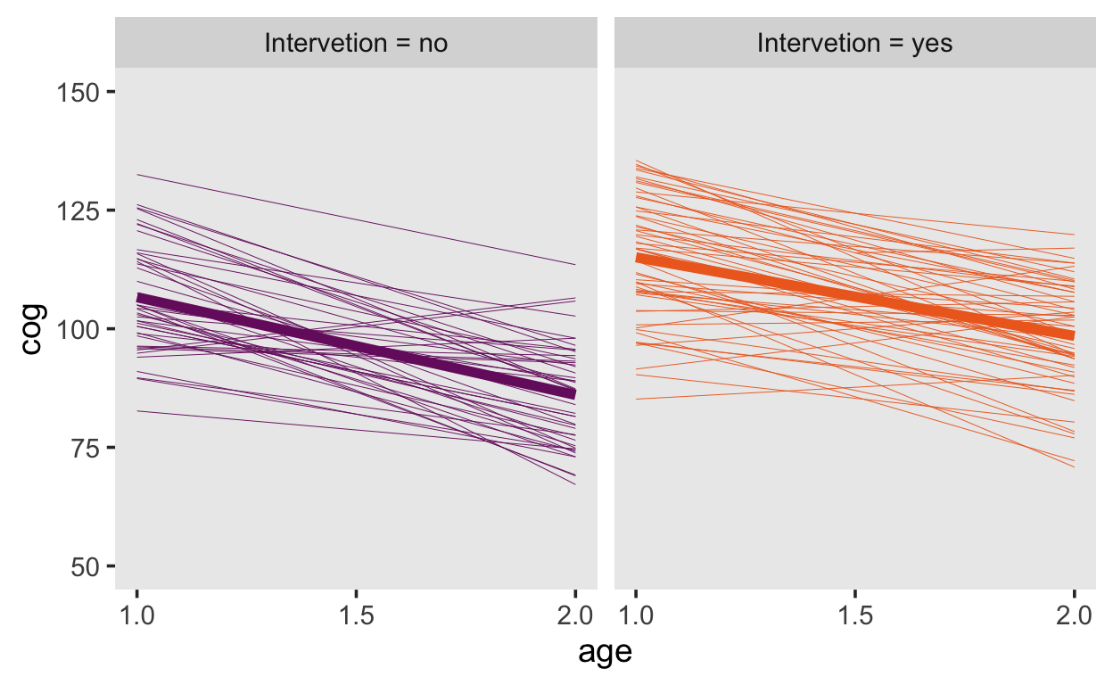
Next, we consider that the children are assigned to two different group.

early_int<-
  early_int|> 
  mutate(label = str_c("Intervetion = ", intervention)) 

early_int |> 
  ggplot(aes(x = age, y = cog, color = label)) +
  stat_smooth(aes(group = id),
              method = "lm", se = F, size = 1/6) +
  stat_smooth(method = "lm", se = F, size = 2) +
  scale_color_viridis_d(option = "B", begin = .33, end = .67) +
  scale_x_continuous(breaks = c(1, 1.5, 2)) +
  ylim(50, 150) +
  theme(legend.position = "none",
        panel.grid = element_blank()) +
  facet_wrap(~label)

Fitting the model with brms

priors_early_1 <- prior(normal(0, 20), class = b)

fit_early_1 <-
  brm(cog ~ 0 + Intercept + age_c + intervention + age_c:intervention + 
        (1 + age_c | id),
      prior = priors_early_1,
      data = early_int,
      control = list(adapt_delta = 0.95),
      seed = 3,
      file = "models/fit_early_1",
      file_refit = "on_change")

fit_early_1

 Family: gaussian 
  Links: mu = identity; sigma = identity 
Formula: cog ~ 0 + Intercept + age_c + intervention + age_c:intervention + (1 + age_c | id) 
   Data: early_int (Number of observations: 309) 
Samples: 4 chains, each with iter = 2000; warmup = 1000; thin = 1;
         total post-warmup samples = 4000

Group-Level Effects: 
~id (Number of levels: 103) 
                     Estimate Est.Error l-95% CI u-95% CI Rhat
sd(Intercept)            9.72      1.17     7.63    12.21 1.00
sd(age_c)                3.90      2.37     0.25     8.72 1.01
cor(Intercept,age_c)    -0.48      0.35    -0.96     0.51 1.00
                     Bulk_ESS Tail_ESS
sd(Intercept)             830     2186
sd(age_c)                 274      498
cor(Intercept,age_c)     2951     1938

Population-Level Effects: 
                      Estimate Est.Error l-95% CI u-95% CI Rhat
Intercept               105.72      1.86   102.02   109.32 1.00
age_c                   -19.92      1.90   -23.66   -16.21 1.00
interventionyes           9.79      2.41     4.91    14.61 1.00
age_c:interventionyes     2.66      2.50    -2.27     7.59 1.00
                      Bulk_ESS Tail_ESS
Intercept                 1247     1818
age_c                     2249     2811
interventionyes           1338     2137
age_c:interventionyes     2395     2714

Family Specific Parameters: 
      Estimate Est.Error l-95% CI u-95% CI Rhat Bulk_ESS Tail_ESS
sigma     8.59      0.50     7.63     9.59 1.01      513     1347

Samples were drawn using sampling(NUTS). For each parameter, Bulk_ESS
and Tail_ESS are effective sample size measures, and Rhat is the potential
scale reduction factor on split chains (at convergence, Rhat = 1).

conditional_effects(fit_early_1,
                    "age_c:intervention")

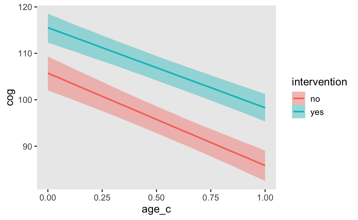
How would you go about demonstrating evidence for or against a difference between the interventions?

Changes in adolescent alcohol use

As part of a larger study of substance abuse, Curran, Stice, and Chassin (1997) collected three waves of longitudinal data on 82 adolescents. Each year, beginning at age 14, the teenagers completed a four-item instrument assessing their alcohol consumption during the previous year. Using an 8-point scale (ranging from 0 = “not at all” to 7 = “every day”), adolescents described the frequency with which they (1) drank beer or wine, (2) drank hard liquor, (3) had five or more drinks in a row, and (4) got drunk. The data set also includes two potential predictors of alcohol use: COA, a dichotomy indicating whether the adolescent is a child of an alcoholic parent; and PEER, a measure of alcohol use among the adolescent’s peers. This latter predictor was based on information gathered during the initial wave of data collection. Participants used a 6-point scale (ranging from 0 = “none” to 5 = “all”) to estimate the proportion of their friends who drank alcohol occasionally (one item) or regularly (a second item).

Do individual trajectories of alcohol use during adolescence differ according to the history of parental alcoholism and early peer alcohol use.

library(tidyverse)

alcohol <- read_csv("https://raw.githubusercontent.com/awellis/learnmultilevelmodels/main/data/alcohol1_pp.csv")
head(alcohol)

# A tibble: 6 x 9
     id   age   coa  male age_14 alcuse  peer  cpeer  ccoa
  <dbl> <dbl> <dbl> <dbl>  <dbl>  <dbl> <dbl>  <dbl> <dbl>
1     1    14     1     0      0   1.73 1.26   0.247 0.549
2     1    15     1     0      1   2    1.26   0.247 0.549
3     1    16     1     0      2   2    1.26   0.247 0.549
4     2    14     1     1      0   0    0.894 -0.124 0.549
5     2    15     1     1      1   0    0.894 -0.124 0.549
6     2    16     1     1      2   1    0.894 -0.124 0.549

Variable	Description
id	subject ID
age	in years
coa	child of alcoholic parent (1 - yes, 0 - no)
male	indicator for male
age_14	age - 14 (0 corresponds to age: 14)
alcuse	alcohol consumption
peer	alcohol use among peers
cpeer, ccoa	centred variables

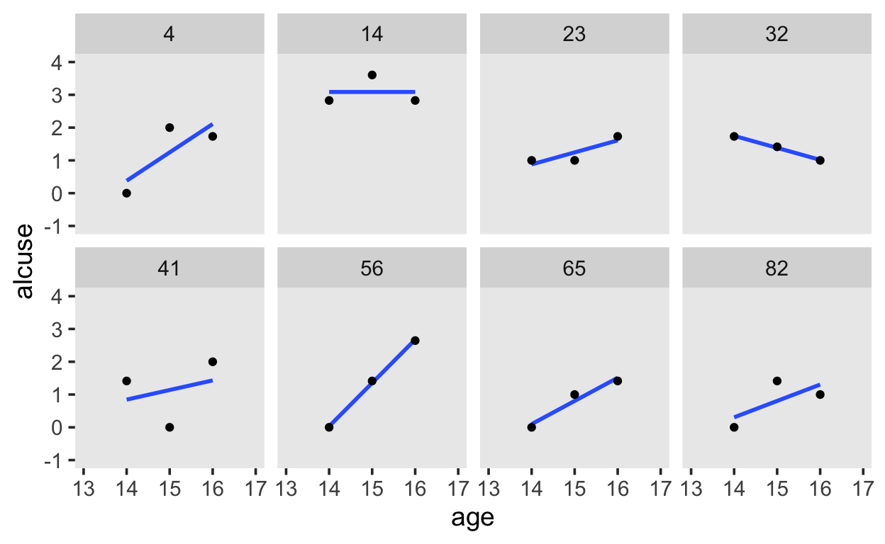
alcohol %>%
  filter(id %in% c(4, 14, 23, 32, 41, 56, 65, 82)) %>%
  
  ggplot(aes(x = age, y = alcuse)) +
  stat_smooth(method = "lm", se = F) +
  geom_point() +
  coord_cartesian(xlim = c(13, 17),
                  ylim = c(-1, 4)) +
  theme(panel.grid = element_blank()) +
  facet_wrap(~id, ncol = 4)

\[\begin{align*} \text{alcuse}_{ij} & = \pi_{0i} + \pi_{1i} (\text{age}_{ij} - 14) + \epsilon_{ij}\\ \epsilon_{ij} & \sim \operatorname{Normal}(0, \sigma_\epsilon^2), \end{align*}\]

\[\begin{align*} \text{alcuse}_{ij} & = \big [ \gamma_{00} + \gamma_{10} \text{age_14}_{ij} + \gamma_{01} \text{coa}_i + \gamma_{11} (\text{coa}_i \times \text{age_14}_{ij}) \big ] \\ & \;\;\;\;\; + [ \zeta_{0i} + \zeta_{1i} \text{age_14}_{ij} + \epsilon_{ij} ] \\ \epsilon_{ij} & \sim \operatorname{Normal} (0, \sigma_\epsilon^2) \\ \begin{bmatrix} \zeta_{0i} \\ \zeta_{1i} \end{bmatrix} & \sim \operatorname{Normal} \begin{pmatrix} \begin{bmatrix} 0 \\ 0 \end{bmatrix}, \begin{bmatrix} \sigma_0^2 & \sigma_{01} \\ \sigma_{01} & \sigma_1^2 \end{bmatrix} \end{pmatrix}, \end{align*}\]

Unconditional means model

\[\begin{align*} \text{alcuse}_{ij} & = \gamma_{00} + \zeta_{0i} + \epsilon_{ij} \\ \epsilon_{ij} & \sim \operatorname{Normal}(0, \sigma_\epsilon^2) \\ \zeta_{0i} & \sim \operatorname{Normal}(0, \sigma_0^2). \end{align*}\]

get_prior(alcuse ~ 1 + (1 | id),
          data = alcohol)

                prior     class      coef group resp dpar nlpar bound
 student_t(3, 1, 2.5) Intercept                                      
 student_t(3, 0, 2.5)        sd                                      
 student_t(3, 0, 2.5)        sd              id                      
 student_t(3, 0, 2.5)        sd Intercept    id                      
 student_t(3, 0, 2.5)     sigma                                      
       source
      default
      default
 (vectorized)
 (vectorized)
      default

fit_alcuse_1 <-
  brm(alcuse ~ 1 + (1 | id),
      data = alcohol,
      file = "models/fit_alcuse_1",
      file_refit = "on_change")

Unconditional growth model

\[\begin{align*} \text{alcuse}_{ij} & = \gamma_{00} + \gamma_{10} \text{age_14}_{ij} + \zeta_{0i} + \zeta_{1i} \text{age_14}_{ij} + \epsilon_{ij} \\ \epsilon_{ij} & \sim \operatorname{Normal} (0, \sigma_\epsilon^2) \\ \begin{bmatrix} \zeta_{0i} \\ \zeta_{1i} \end{bmatrix} & \sim \operatorname{Normal} \begin{pmatrix} \begin{bmatrix} 0 \\ 0 \end{bmatrix}, \begin{bmatrix} \sigma_0^2 & \sigma_{01} \\ \sigma_{01} & \sigma_1^2 \end{bmatrix} \end{pmatrix}. \end{align*}\]

get_prior(alcuse ~ 0 + Intercept + age_14 + (1 + age_14 | id),
          data = alcohol)

                prior class      coef group resp dpar nlpar bound
               (flat)     b                                      
               (flat)     b    age_14                            
               (flat)     b Intercept                            
               lkj(1)   cor                                      
               lkj(1)   cor              id                      
 student_t(3, 0, 2.5)    sd                                      
 student_t(3, 0, 2.5)    sd              id                      
 student_t(3, 0, 2.5)    sd    age_14    id                      
 student_t(3, 0, 2.5)    sd Intercept    id                      
 student_t(3, 0, 2.5) sigma                                      
       source
      default
 (vectorized)
 (vectorized)
      default
 (vectorized)
      default
 (vectorized)
 (vectorized)
 (vectorized)
      default

fit_alcuse_2 <-
  brm(alcuse ~ 0 + Intercept + age_14 + (1 + age_14 | id),
      prior = c(prior(normal(0, 15), class = b)),
      data = alcohol,
      file = "models/fit_alcuse_2")

Effect of COA

\[\begin{align*} \text{alcuse}_{ij} & = \gamma_{00} + \gamma_{01} \text{coa}_i + \gamma_{10} \text{age_14}_{ij} + \gamma_{11} \text{coa}_i \times \text{age_14}_{ij} + \zeta_{0i} + \zeta_{1i} \text{age_14}_{ij} + \epsilon_{ij} \\ \epsilon_{ij} & \sim \text{Normal} (0, \sigma_\epsilon^2) \\ \begin{bmatrix} \zeta_{0i} \\ \zeta_{1i} \end{bmatrix} & \sim \text{Normal} \begin{pmatrix} \begin{bmatrix} 0 \\ 0 \end{bmatrix}, \begin{bmatrix} \sigma_0^2 & \sigma_{01} \\ \sigma_{01} & \sigma_1^2 \end{bmatrix} \end{pmatrix}. \end{align*}\]

fit_alcuse_3 <-
  brm(data = alcohol,
      alcuse ~ 0 + Intercept + age_14 + coa + age_14:coa + (1 + age_14 | id),
      prior = c(prior(normal(0, 15), class = b)),
      file = "models/fit_alcuse_3")

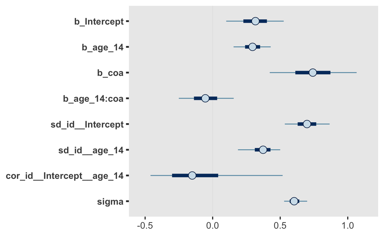
fit_alcuse_3

 Family: gaussian 
  Links: mu = identity; sigma = identity 
Formula: alcuse ~ 0 + Intercept + age_14 + coa + age_14:coa + (1 + age_14 | id) 
   Data: alcohol (Number of observations: 246) 
Samples: 4 chains, each with iter = 2000; warmup = 1000; thin = 1;
         total post-warmup samples = 4000

Group-Level Effects: 
~id (Number of levels: 82) 
                      Estimate Est.Error l-95% CI u-95% CI Rhat
sd(Intercept)             0.70      0.10     0.51     0.90 1.01
sd(age_14)                0.36      0.09     0.15     0.52 1.02
cor(Intercept,age_14)    -0.10      0.29    -0.50     0.70 1.01
                      Bulk_ESS Tail_ESS
sd(Intercept)              947     2048
sd(age_14)                 341      668
cor(Intercept,age_14)      624      601

Population-Level Effects: 
           Estimate Est.Error l-95% CI u-95% CI Rhat Bulk_ESS
Intercept      0.32      0.13     0.06     0.57 1.00     2454
age_14         0.29      0.08     0.13     0.46 1.00     3114
coa            0.74      0.19     0.36     1.12 1.00     2196
age_14:coa    -0.05      0.12    -0.29     0.19 1.00     2956
           Tail_ESS
Intercept      2757
age_14         2854
coa            2481
age_14:coa     2883

Family Specific Parameters: 
      Estimate Est.Error l-95% CI u-95% CI Rhat Bulk_ESS Tail_ESS
sigma     0.61      0.05     0.52     0.72 1.01      524     1151

Samples were drawn using sampling(NUTS). For each parameter, Bulk_ESS
and Tail_ESS are effective sample size measures, and Rhat is the potential
scale reduction factor on split chains (at convergence, Rhat = 1).

mcmc_plot(fit_alcuse_3)

loo_alcuse_2 <- loo(fit_alcuse_2)
loo_alcuse_3 <- loo(fit_alcuse_3)

loo_compare(loo_alcuse_2, loo_alcuse_3)

             elpd_diff se_diff
fit_alcuse_2  0.0       0.0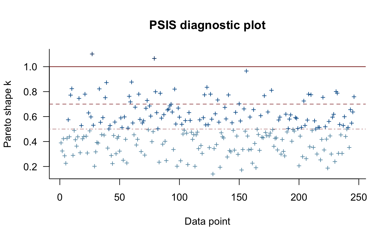   
fit_alcuse_3 -0.7       2.4

plot(loo_alcuse_3)

Time-varying predictors

If we have time-varying predictor variable, it is a good idea the decompose these into a subject’specific mean (trait) and a session-by-session deviation from that mean (state).

Let’s look at some simulated data, in which patient are assigned to either a control or a therapy (ACT) group. Patients’ wellbeing (score) is assessed over the course of 12 sessions. In addition, we have the patient-rated therapeutic alliance, which reflects how the quality of patient-therapist interactions.

wellbeing <- read_csv("https://raw.githubusercontent.com/awellis/learnmultilevelmodels/main/data/wellbeing.csv")

wellbeing |> 
  ggplot(aes(session, score, color = therapy)) +
  geom_line() +
  geom_point() +
  geom_line(aes(session, alliance), linetype = 2) +
  scale_x_continuous(breaks = seq(2, 12, by = 2)) +
  scale_color_brewer(type = "qual") +
  facet_wrap(~patient)

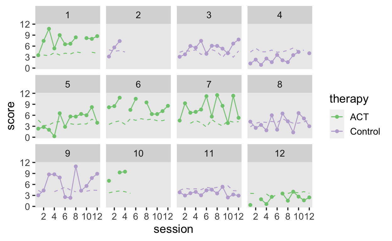
We want to predict patient’s wellbeing as a function of the therapeutic alliance, while accounting for a linear trend.

How would you specify this model, as well as unconditional models?
At which level is the predictor variable alliance?

Decomposing time-varying predictors

Instead of using the raw alliance variable, we will create two new variables: the average alliance, and the session-by-session deviations from the average. The average will be a patient-level (level 2) predictor, and can be used to explain variability between patients, whereas the deviations reflect fluctuations within patients at individual sessions.

wellbeing <- wellbeing |> 
  group_by(patient) |> 
  mutate(al_between = round(mean(alliance, na.rm = TRUE), 2),
         al_within = alliance - al_between)

fit_alliance_1 <- brm(score ~ session + (1 + session| patient),
                    data = wellbeing,
                    file = "models/fit_alliance_1")

fit_alliance_2 <- brm(score ~ session + al_between + al_within + 
                      (1 + session  + al_within | patient),
                    data = wellbeing,
                    file = "models/fit_alliance_2")

fit_alliance_3 <- brm(score ~ session + al_within + 
                      (1 + session  + al_within | patient),
                    data = wellbeing,
                    file = "models/fit_alliance_3")

fit_alliance_2

 Family: gaussian 
  Links: mu = identity; sigma = identity 
Formula: score ~ session + al_between + al_within + (1 + session + al_within | patient) 
   Data: wellbeing (Number of observations: 111) 
Samples: 4 chains, each with iter = 2000; warmup = 1000; thin = 1;
         total post-warmup samples = 4000

Group-Level Effects: 
~patient (Number of levels: 12) 
                         Estimate Est.Error l-95% CI u-95% CI Rhat
sd(Intercept)                2.67      0.73     1.58     4.34 1.00
sd(session)                  0.09      0.07     0.00     0.27 1.00
sd(al_within)                0.90      0.57     0.05     2.21 1.00
cor(Intercept,session)      -0.14      0.46    -0.87     0.80 1.00
cor(Intercept,al_within)    -0.37      0.44    -0.96     0.67 1.00
cor(session,al_within)      -0.11      0.49    -0.89     0.84 1.00
                         Bulk_ESS Tail_ESS
sd(Intercept)                1566     2500
sd(session)                  1304     1738
sd(al_within)                1661     1780
cor(Intercept,session)       2799     2463
cor(Intercept,al_within)     2895     2439
cor(session,al_within)       2263     3065

Population-Level Effects: 
           Estimate Est.Error l-95% CI u-95% CI Rhat Bulk_ESS
Intercept      4.89      8.00   -10.44    21.29 1.00     1426
session        0.18      0.06     0.05     0.30 1.00     3139
al_between    -0.11      1.88    -3.94     3.54 1.00     1440
al_within     -0.72      0.50    -1.72     0.22 1.00     2778
           Tail_ESS
Intercept      1882
session        2514
al_between     1880
al_within      2668

Family Specific Parameters: 
      Estimate Est.Error l-95% CI u-95% CI Rhat Bulk_ESS Tail_ESS
sigma     1.80      0.14     1.55     2.10 1.00     3490     2939

Samples were drawn using sampling(NUTS). For each parameter, Bulk_ESS
and Tail_ESS are effective sample size measures, and Rhat is the potential
scale reduction factor on split chains (at convergence, Rhat = 1).

Kurz, A. Solomon. 2021. Applied Longitudinal Data Analysis in Brms and the Tidyverse. Version 0.0.2. https://bookdown.org/content/4253/.

RAUDENBUSH, STEPHEN W., and WING-SHING CHAN. 1992. “Growth Curve Analysis in Accelerated Longitudinal Designs.” Journal of Research in Crime and Delinquency 29 (4): 387–411. https://doi.org/10.1177/0022427892029004001.

Singer, Judith D., and John B. Willett. n.d. Applied Longitudinal Data Analysis: Modeling Change and Event Occurrence. Applied Longitudinal Data Analysis. Oxford University Press. Accessed June 10, 2021. https://oxford.universitypressscholarship.com/view/10.1093/acprof:oso/9780195152968.001.0001/acprof-9780195152968.

Longitudinal Models

Exploring data

Early Intervention

Fitting the model with brms

Changes in adolescent alcohol use

Unconditional means model

Unconditional growth model

Effect of COA

Time-varying predictors

Decomposing time-varying predictors

References

Corrections

Reuse

Citation